We may be compensated for your purchase of any of the products featured on this page – it helps us keep the lights on :)
A Linked Picture in Excel is one that displays the contents of another cell(s) in real-time. When you create a Linked Picture, you create a sort of live feed to content in other cells. Making this an excellent tool to help you monitor other cells and can add an interesting visual to your spreadsheet.
The other cells can be in the same workbook or a different one.
While you can change the appearance of Linked Pictures, typically, you would want them to mirror the copied cell.
Think of Linked Pictures as a live cam of another cell or range of cells in Excel.
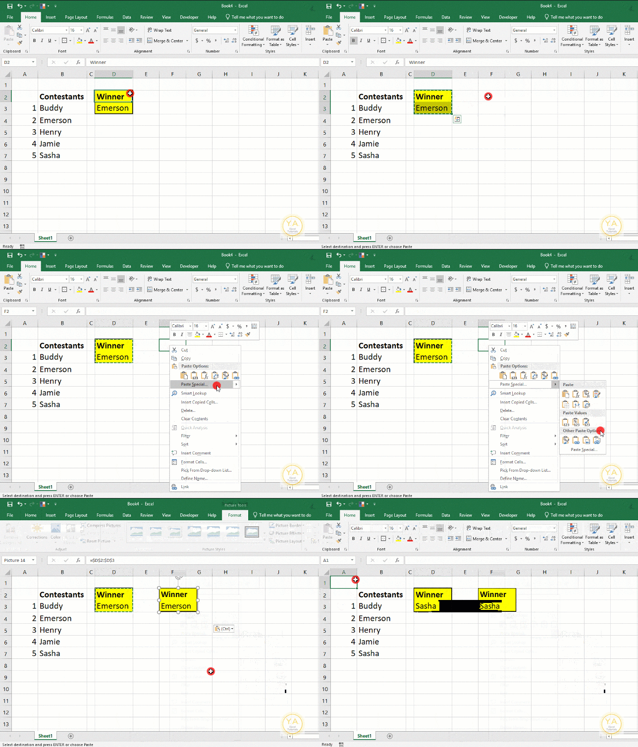
How do you know if your Picture is linked? You’ll see this in the Formula Bar. Select your Linked Picture or Shape and you should see the cell or cell range displayed in the Formula Bar.
NOTE: Linked Pictures can take up a lot of memory in a spreadsheet. Having too many could bog down your workbook.
3 Ways to Create a Linked Picture in Excel
1. Paste a Cell or Range of Cells as a Linked Picture
You can make a Linked Picture using Copy and a Paste Special option.
Simply select the cell or cells you want to view in the Linked Picture, Copy and, in Paste Special, select Linked Picture.
This will create a Linked Picture of the cell(s) you just copied!

Keep in mind that, because this captures the area as it is displayed, you’ll likely see any gridlines inside of your Linked Picture. To avoid this, uncheck Gridlines in your View tab.
2. Use Excel’s Camera Tool to Create a Linked Picture
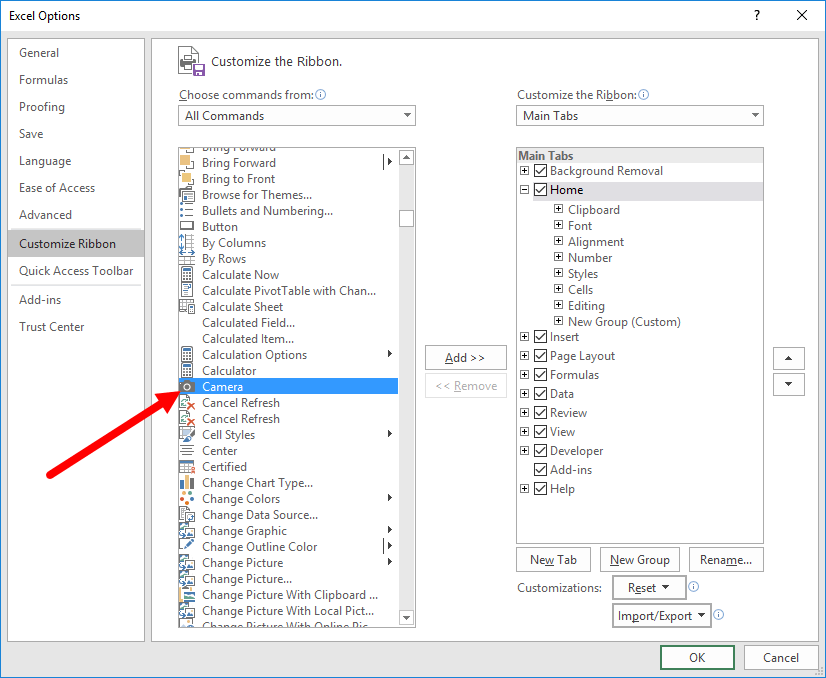
The first thing you’ll want to do is make sure you have the Camera Tool available. It should be in your Ribbon.

If you don’t see it, go to your File / Options / Customize Ribbon (or Quick Access Toolbar if you want to add it there) / Change the drop down to All Commands and then scroll until you see Camera. Click Add, then OK.

Next, highlight the area that you want to capture for your Linked Picture.
After highlighting the area that you want, simply click on the Camera button.
Then click where you would like to place your Linked Picture and it will automatically Paste.
As with the Paste Special option, if you see any gridlines inside of your Linked Picture, uncheck Gridlines in your View tab.
3. Manually Link a Shape to a Cell
Maybe you don’t need to mirror other cells. If you simply want to display the contents, a formula result, for example, of a single cell in a Shape, you can easily do this too!
Simply select the Shape and, in the Formula Bar, type = then select the cell you want to reference.

Simple as that!
Then, you can format the Shape and any text or numbers inside the Shape as you normally would.
How to Edit Your Linked Picture
In most cases, a square or rectangle that mirrors the original cell(s) will suffice, but if you want to, you can change the Shape of your Linked Picture.
To do so, you’ll need the Change Shape tool.

If you don’t see it, go to your File / Options / Customize Ribbon / Change the drop-down to All Commands and then scroll until you see Change Shape. Click Add, then OK.

You can also use the Picture Tools / Format options to change the color, style, size, etc of your picture.


How can I make a picture in a certan cell to auyo appear in other cells without paste in cells manually?
How can I make a picture in a certan cell to auto appear in other cells without paste in cells manually?