We may be compensated for your purchase of any of the products featured on this page – it helps us keep the lights on :)
If you’ve tried to combine text with numbers in Excel and keep the formatting, you’ve likely found that it is not always as straightforward as it may seem.
For example, if you try to join text with numbers like dates, time, percentages, etc, you often end up with results that are hard to decipher.
Your solution? Use the TEXT function.
The TEXT function in Excel converts numbers to text using custom formatting. And you can use it when you want to combine numerical values or formula results with other text while keeping the formatting you want. Here’s how:
How to Use the TEXT Function in Excel
Watch: TEXT Function in Excel – Tutorial
To use the TEXT function, you need to enter 2 pieces of information:
- a numerical value to be converted to text
- the custom format you want applied to the resulting text
For example, say you want to reference a cell displaying a time value that updates periodically and join it with text that reads “We meet at: “.
Pretend the cell is currently displaying 8:00 AM.
Simply concatenating the text with the time value would result in “We meet at: 0.3333”
Few people would find this helpful.
The issue is that simply combining the 2 cells ends up in the entire result using a single style of formatting.
For this example, you would need the text to remain as text, but time value to be formatted so that it displays as, well…time.
Enter the TEXT function.
The TEXT function converts cell contents to text while applying custom formatting to its result.
In this example, you would use the TEXT function to apply a time format to the cell containing the time value.
It would look like this:
=TEXT(A1,”h:mm AM/PM”)
*Where cell A1 contains the time.
NOTE: Because the TEXT function converts its results to text, the formatting settings needs to be inside quotation marks.
You can then use the ampersand “&” to join it with other text.
=”We meet at: “&TEXT(A1,”h:mm AM/PM”)
And the final result would be:
We meet at: 8:00 AM
TIP: The quotation marks can be a bit touchy. For example, mine only work when I type them using my laptop’s keyboard. The quotation marks on my phone’s keyboard are formatted differently and don’t work.
How do you know what formatting to use in the TEXT function?
Knowing how to input the format style into the TEXT function is the trickiest part.
In the example above, the custom formatting is the part that reads: “h:mm AM/PM“
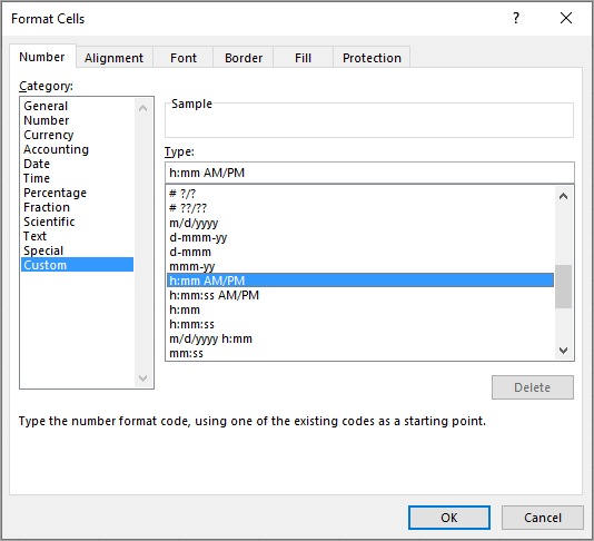
The formatting you’ll enter here should be typed the same as what would be used in the Format Cells dialog box. You can right-click on any cell and select “Format Cells” to open this.

What to do when you don’t know the format settings
One way you can figure out the format settings to use in your TEXT function is by applying the formatting you need to a cell (any cell) using the options in the Format Cells tool.
To do this, in the Format Cells tool, select the category you need from the left side. Then choose which of the available formatting options you want to use.
Then, place your cursor in the cell you just formatted, right-click, and open Format Cells again.
This time, go to the Custom category. You should see in the “Type” field the formatting code used in the cell.
You can now copy this to use in your TEXT function!
FYI: the Type field may also display some other gibberish just before the settings you need, but you can ignore that when entering it in your TEXT function.
For more on creating your own custom formatting, take a look at this list from Microsoft to help you with the settings used in the Format Cells box.
FYI, this was created using the desktop version of Excel in Microsoft 365.


Leave a Reply