We may be compensated for your purchase of any of the products featured on this page – it helps us keep the lights on :)
Did you know you can change the gridline color in Excel spreadsheets? This is a great option to help your worksheets stand out or for color-coding.
Say you have a workbook with multiple sheets and each represents something different, changing the color of the gridlines can help with your color-coding.
There are a couple of ways to do this and both are pretty simple to do!
How to Change the Color of the Gridlines in your Excel Spreadsheet
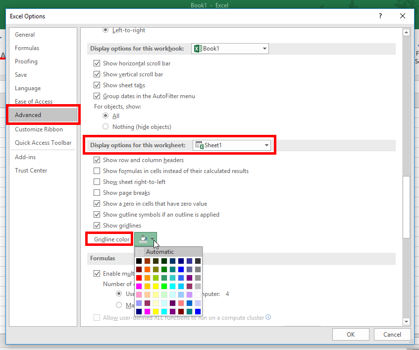
1. Change the Gridline Color using the “Gridline Color” setting in your Excel Options
If your spreadsheet is open, select “File” – this located to the left of your Home tab.
Then, select “Options.”

Next, scroll to “Advanced” on the menu to the left side of the screen.
Then find “Display Options for this Worksheet.”
Once in the Display Options, select the tab you’d like to color the gridlines for and choose your gridline color.
Click OK and your gridlines will now be in a new color!

What to know about coloring your gridlines from the Options menu
There are a few things to keep in mind when recoloring your gridlines this way.
First, you’re not able to enter specific RBG colors. So, if there is a specific brand color you need to use, you won’t be able to. However, all the standard color options are available so you still have a good variety to choose from.
This only recolors the gridlines for one worksheet at a time (i.e., one tab at a time). So, you’ll need to repeat this for each tab that you want to color the gridlines for.
Because the color applies only to one sheet at a time, this will not carry over to other workbooks.
However, if you want to save this so you can reuse it, you can create an Excel template of a blank sheet with gridlines already colored!
If you need to use a specific color or color multiple sheets at the same time, try this instead:
2. Color Excel Sheet Gridlines Using the Borders Options
With this next option, you can color the gridlines in your spreadsheet using one of the standard colors or a specific color, like for when you need to use a brand color.
To do this, it’s easier to set the format you want for your gridlines first.
TIP: To color the gridlines for multiple sheets at the same time, make sure to select the tabs for all the sheets you want to recolor before you begin.
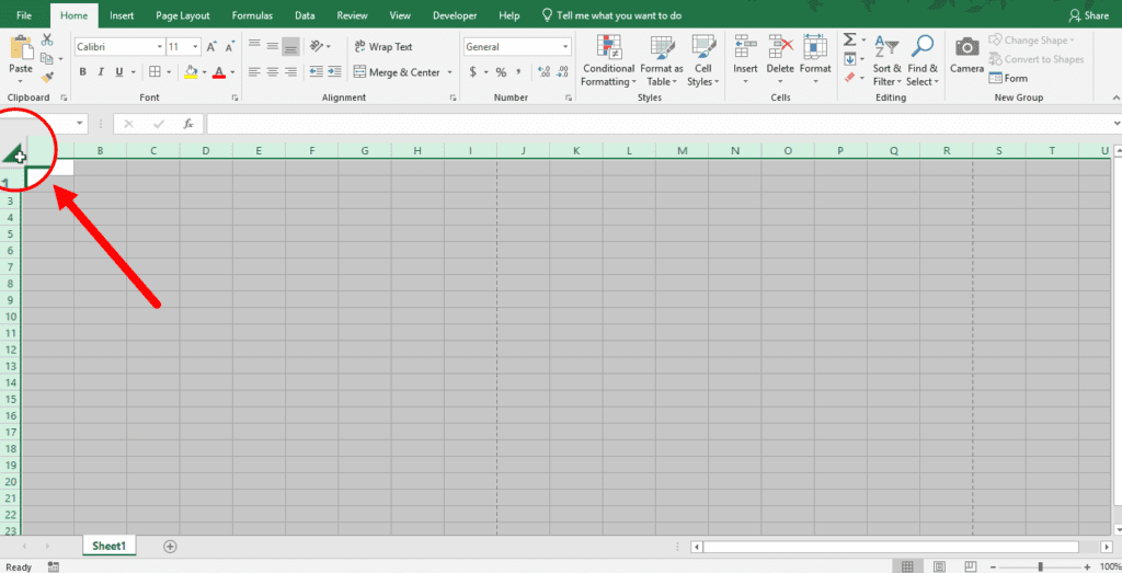
Begin by selecting your entire spreadsheet. Use either Ctrl+A or select the spreadsheet by clicking on the triangle on the top left corner of your sheet.

Once your sheet is selected, in your Home tab, click on the “Borders” icon.
Scroll to “Line Color” and select a color from the options or set your own color by selecting “Custom Color.”

If you want to make your grid lines bolder, thicker or use a different line style altogether, pressing the “Gridlines” button again, select “Line Style” and select the style of line you’d like to use.

Finally, select the “Borders” icon again, making sure that it’s set to “All Borders.”

Your Gridlines will now be a new color!

To save and reuse, create an Excel template of a blank sheet with gridlines already colored!

Leave a Reply