Hidden Rows and Columns in Excel: The Art of Concealment

We may be compensated for your purchase of any of the products featured on this page – it helps us keep the lights on :)

The Hide feature in Excel is an easy way to hide and unhide rows and columns of data that you don’t want to display on your sheet. This can help you focus only on what you need at any given moment.

But hiding can also make you forget something is there – i.e., “out of sight, out of mind.”

NOTE: Hiding rows or columns in Excel does not delete them!!!

I never want you to be caught accidentally sharing confidential information! – Ugh! What a nightmare!

Read below to learn all about hidden rows and columns in Excel to help you avoid this kind of mishap.

Hidden Rows and Columns: All About the Hide Feature in Excel

What are hidden rows or columns in Excel?

The term “hidden row” or “hidden column” in Excel refers to a row or column that is hidden from view.

Data contained in hidden rows or columns is not deleted, it is only hidden from view.

This is why it is important to delete any sensitive information that you do not want others to see. Simply hiding it makes it easy to access.

You Might Like: How to Protect Cells in Excel – Tutorial

Why would you want to hide rows or columns?

Spreadsheets can get cumbersome with large data sets, charts, links, and just a lot of stuff to look at!

I don’t know about you, but sometimes I look at a spreadsheet with a ton of data and my head starts spinning even before I do any work!

Hiding rows and columns is one of many tools that you can use to help you clean up a spreadsheet to make it easier to focus on key parts.

For example, if you’re looking at data by year and you’re interested in only 2022 data, perhaps you hide any columns or rows containing data from 2021.

How to hide rows or columns in Excel?

There are a few ways that you can hide rows or columns in Excel.

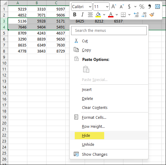
One common way is to select the entire row or column that you want to hide, right-click, and select “Hide” from the options.

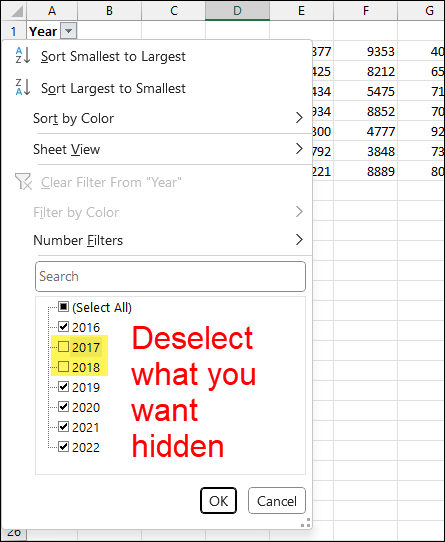
Another popular option is to apply a filter to your data. Any items that are unselected for the filter (i.e., filtered out) will be hidden from view.

How to find hidden rows or columns in a spreadsheet?

What if you’ve forgotten what you previously hid on your sheet? Or have just received a spreadsheet that you think may have hidden data?

It’s important to search for hidden data for a few reasons:

1. If using subtotals, like a filter would, hidden data can affect any calculations. Thus, affecting results you might need for decision-making.
2. You might need to have knowledge of the hidden data. Without unhiding it, you may never know it is.

There are a few ways that you can use to find if there are hidden rows or columns in an Excel spreadsheet.

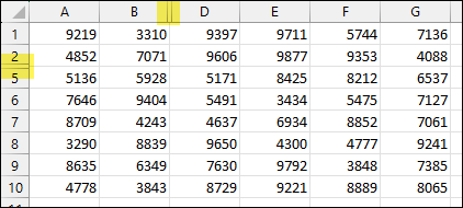
In the image below, column C and rows 3 and 4 are hidden.

You can tell they are hidden in a few ways:

1. Look for the missing label: The letter C is missing along the columns (on the top) and the numbers 3 and 4 are missing along the row numbers (along the left side of the sheet).
2. Look for “double bars” along the column and rows: Where the column is hidden and where the rows are hidden, you’ll find a sort of double bar where there would normally be only a single bar separating each row and column. This is highlighted in yellow in the image below.

• Use the “Go to Special” feature: You can use the Go to Special feature to highlight visible cells. This helps find hidden cells by displaying a whiteish line where hidden rows or columns are.

You can find the “Go to Special” feature in your Excel Ribbon in the Home tab, in the Editing section. Once here click on Find & Select, then click on Go to Special, and select Visible Cells Only from the pop-up window.

Alternatively, you can use the Ctrl+F keyboard shortcut, then select Visible Cells Only.

• Use the Inspect Document feature: The Inspect Document feature lets you inspect your spreadsheet for multiple items. For this example, we’re only focusing on hidden rows and columns.

TIP: Save your document before using this feature.

While this feature doesn’t tell you which rows or columns are hidden, it will tell you how many are in your document.

You can find the Inspect Document feature in the File tab of your Excel Ribbon, in the Info section. Once here, click on Inspect Workbook, then click on Inspect Document.

Select “Yes” or “No” to save or not save your document before proceeding.

The Document Inspector window will now open. Once here, make sure that Hidden Rows and Columns is selected. Click “Inspect.”

How to Unhide Rows or Columns in Excel

An easy way to display, or unhide, any hidden rows, is to select the rows surrounding the hidden rows, right-click, and select “Unhide” from the options.

Likewise, to unhide hidden columns, select the columns surrounding the hidden ones, right-click, and select “Unhide.”

You can also double-click on any “double bars” to unhide them.

If using a filter and the data has been “filtered-out,” you’ll need to select the filtered items to unhide them.

How to Delete Hidden Rows or Hidden Columns in Excel

If your spreadsheet contains sensitive information, or just data your recipient may not need, it is best practice to delete any hidden rows or columns before sharing.

Otherwise, your recipient can access your hidden data by simply unhiding it.

IMPORTANT: Make sure you have saved what you need before deleting!

To delete hidden rows or columns, you can:

1. Manually delete any rows, columns, or clear the data in specific cells
2. You can also use the Inspect Document feature to delete all hidden rows or columns at once

Once you’ve run the Inspect Document tool, the results will display the number of hidden rows and columns in your workbook.

To remove all of them in one go, simply click the “Remove All” button in the inspection results window.

NEXT: Insert Messages in Excel – 5 ways!

FYI: This tutorial was created using the desktop version of Excel in Microsoft 365.