Ways to Link Sheets in Same Excel Workbook (+ video tutorial)

We may be compensated for your purchase of any of the products featured on this page – it helps us keep the lights on :)

If you use Excel, you’ll inevitably need to link sheets in a workbook. Let’s go over different ways you can do this.

4 Ways You Can Create a Link Between Tabs in a Workbook

WATCH: Ways to Link Sheets in an Excel Workbook – Tutorial

1. Use the Equal sign to create a reference to a cell

Probably the most common way to link cells from different sheets is by using the equal sign to create a cell reference.

To do this, type the equal sign. Then go to the sheet that has the cell you want to link to, select it, and press Enter.

For example, if you’re in Sheet1 of your workbook and you link to a cell in Sheet2, your link would look something like this:

=Sheet2!A1

2. Use the Paste Link feature to create a link to a data range

One of the fastest ways you can create a link to a set of data is by using the Paste Link feature.

To use this feature:

• Go to the sheet with the cells you want to link to and copy them
• Place your cursor where you want to paste the linked data and right-click
• In the Paste options either
  • Select the icon with the links or
  • Click on Paste Special then
    • Click on Paste Link

3. Create a link to a named range

If your worksheet contains named ranges, you can create a link to these by referencing the named range.

Here’s how:

1. Place your cursor where you want to paste the link to the named range and type an equal sign
2. Begin typing the name of the named range, select it, then press Enter to populate it on your sheet

Important note about creating links to named ranges:

Linking named ranges works a little different than other methods. This is because the linked cells populate as a group.

If you place cursor on any of the values, you’ll see a light blue box around your linked range of cells.

Because of this grouping, you cannot delete individual values from the range. You would need to select the entire range and press Delete.

You also cannot change any of the values. Doing will result in an error.

4. Create a hyperlink to another sheet

You can also create a hyperlink to another sheet. While this won’t display the values from the cell you’re linking to, it will let you jump to that location.

To create a hyperlink, place your cursor in the cell where you’d like your hyperlink. Then, either right-click and select “Link” or press Ctrl+K on your keyboard.

This will open a window with options for your hyperlink.

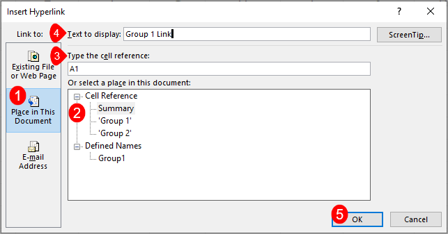
1. In the “Link to” section, select “Place in this Document”
2. From the “Select a Place in this Document” section, select the sheet you want to link to or a Named Range if you have some.
3. The “Cell Reference field” displays where in the linked sheet your hyperlink will jump to. Unless you selected a named range, the link will default to cell A1 of the linked sheet. You can change this here, if you like.
4. The “Text to Display” field shows you what your link will be labeled. You can leave it as is or type something friendlier.
5. Press Ok to create your hyperlink.

What if, instead, you want to link values from different sheets so that you can do calculations??? Here are 4 ways you can do this:

4 Ways to Calculate Values Across Sheets in a Workbook

WATCH: Ways to Link Sheets in an Excel Workbook – Tutorial

1.     Insert a calculation symbol between linked cells

You can link to cells in different sheets of your workbook and run a calculation by inserting a calculation symbol (+ * – / ) between each cell reference.

To do this:

1. type the equal sign
2. go to the sheet that has the first cell you want to link to for your calculation and select it
3. type the calculation symbol you need
4. select the next cell for your calculation
5. type the calculation symbol
6. repeat to include additional cells
7. press Enter when done

For example, if you’re in Sheet1 of a workbook, you can add the values in cells A1 and A2 of Sheet2 with a formula like this:

=Sheet2!A1+Sheet2!A2

2.     Use a function to calculate between sheets

Instead of using a bunch of symbols to calculate between linked sheets, you can also use a function.

For example, to add values from different sheets, you can:

1. type =Sum(
2. select the first cell you want to include
3. add a comma
4. select the next cell
5. add another comma and so on
6. press Enter when done

It would look something like this:

=SUM(Sheet2!A1,Sheet3!A1,…)

3.     Use a 3D formula to calculate values across sheets

3D formulas work by referencing the same cell locations across multiple, adjacent sheets.

This means that all the values you are calculating need to be in the same cell locations in all the sheets you’re referencing.

AND the sheets you are referencing need to all be adjacent to each other.

For instance, you could include Sheet2, Sheet3, and Sheet4 in your 3D formula, but could not omit Sheet3.

For example, to do a 3D formula for adding:

1. type =SUM(
2. select the cell or cell range you want to link for your calculation
3. while holding down the Shift key, select each of the other tabs that you want to include in the calculation (you could also select only the first and last tabs. The others will be included by default)
4. press Enter when done

Your 3D formula should look something like this:

=SUM(Sheet2:Sheet3!A1)

4.     Consolidate data across sheets in your workbook

You can summarize data across sheets by using the Consolidation feature.

To consolidate, you’ll need to make sure that the cell ranges you are selecting are laid out the same way. They don’t have to be in the exact same location in the sheet, like for the 3D formula, but they do need to have the same type of data and layout.

TIP: It’s also a good idea to create your consolidation in a blank sheet. If you select to link to your original data, Excel will group your data. This requires a blank area.

You’ll find the Consolidate feature in the Data tab, in the Data Tools section.

Click on Consolidate. Then:

• Select the type of calculation you want for your consolidation

• Next, select the first range of cells to include in the calculation

TIP: If you want to use your column and/or row headers as labels in your consolidation, make sure to include them when you select your data ranges.

• Click Add
• Repeat until all ranges you want to be included have been selected
• Select whether you’d like to use your existing column and/or row headers to label your consolidation results

• Select if you want to create a link to the original data or not

If not, you will see only a result for the calculation you selected.

If you select to create links to the original data, your results will be automatically grouped. You can then toggle displaying the group detail on and off.

---

FYI, this was created using the desktop version of Excel in Microsoft 365.

---