How to Use the RANDARRAY Function to Generate Random Data in Excel (+ video tutorial)

We may be compensated for your purchase of any of the products featured on this page – it helps us keep the lights on :)

If you use Microsoft 365 or Excel 2021, the RANDARRAY function just made generating random data sets in Excel a whole lot easier! Let’s take a look at this function.

What is the RANDARRAY function?

RANDARRAY is a dynamic array function that combines the features of the RAND and RANDBETWEEN functions, then adds even more tricks!!!!

So, what do I mean by this?

Like Excel’s RAND and RANDBETWEEN, RANDARRAY is a dynamic function that generates random numbers.

NOTE: a dynamic function is one that regenerates its result any time any change is made in the sheet.

But, unlike its predecessors, with RANDARRAY you can create random numbers to fill entire cell ranges in one go and more! All in a single formula.

With RANDARRAY, you can:

• Use it like the RAND function to generate a single random number
• Set the quantity of random numbers to generate by setting the number of rows and columns you want
• Establish minimum and maximum limits to the random numbers generated – as you would with RANDBETWEEN
• Set whether you want to see your results as decimals or as integers

This makes RANDARRAY the easiest way to generate large data sets of random values quickly!

Why use RANDARRAY???

RANDARRAY is customizable. You can use it to generate random numbers in whatever size range you want. For example, you could set an area that is 4 rows long and 10 columns wide.

It’s efficient for creating large data sets. You no longer need to copy and paste the RAND or RANDBETWEEN functions over and over. You can now do it all in a single formula, saving you time.

Likewise, if you need to edit the settings in the formula, you only need to do it once and it will affect all its results!

RANDARRAY is a dynamic array function. This means that, by inputting the function in a single cell, you can apply (or “spill”) its results to multiple, blank neighboring cells.

How to use RANDARRAY in Excel to Generate Random Numbers

With all the gushing and excitement for this function out of the way, let’s get to how you would use RANDARRAY!

The full RANDARRAY function is =RANDARRAY([rows],[columns],[min],[max],[integer])

Depending on what results you’re looking for, you may or may not need to use any of these fields. Wild, right?! Let’s look at some examples.

Insert a Single Random Value in Only One Cell

If you want to generate a single random number in a cell, as you would have with the old RAND function, you would simply type =RANDARRAY() and a random number between 0 and 1 will be generated for you.

Set the Number of Rows and/or Columns to Insert Random Numbers In

RANDARRAY makes it easy to set the quantity of random numbers generated; it has inputs for the number of rows and columns you want the results to be in.

You’ll find this option in the first two arguments of the function: =RANDARRAY([rows],[columns],[min],[max],[integer])

Here are some examples:

Use RANDARRAY to Insert Random Values in Rows Only

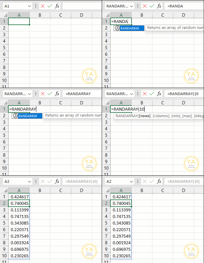
Let’s say you want to apply random values to the 10 rows below the cell in which you type the function, you would use: =RANDARRAY(10)

Use RANDARRAY to Insert Random Values in Columns Only

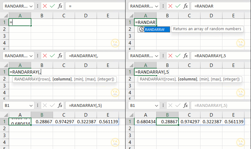
To insert random values into only the 5 columns to the right of your active cell, you would need to use a comma to “skip” over the first argument and type the number 5 for the second argument. Like this: =RANDARRAY(,5)

Set the Number of Rows and Columns to Include in the RANDARRAY Results

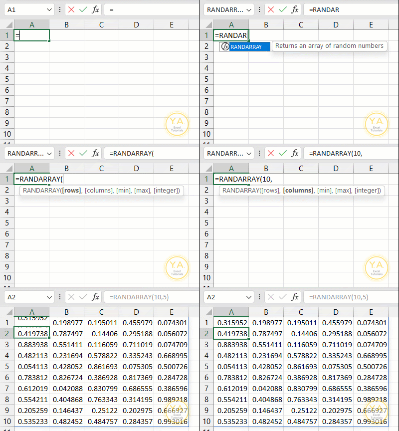
You can probably guess the next example! To insert random values into an area made up of 10 rows and 5 columns, you would type: =RANDARRAY(10,5)

Set Minimum and Maximum Values in RANDBETWEEN

Like in RANDBETWEEN, with RANDARRAY you can set minimum and maximum values for your random numbers.

You’ll find this option in the third and fourth arguments of the function: =RANDARRAY([rows],[columns],[min],[max],[integer])

Building on our last example, let’s say that we want for the random values in our 10 x 5 cell range to be no less than 200 and no more than 750. Our formula would look like: =RANDARRAY(10,5,200,750)

Set Your RANDARRAY results as Decimals or as Integers

With the final argument, you can set if you’d like for the results of the RANDARRAY function to be decimals or integers:

=RANDARRAY([rows],[columns],[min],[max],[integer])

The default for the function is decimal values (as you could probably tell by the results in our earlier examples).

This means that, if you want your results to be in decimal form, you can just press Enter and skip this argument altogether.

But, if you want for your random values to be integers, you’ll need to select that in your final argument. You can do so by either typing “False” or the number “2.”

=RANDARRAY(10,5,200,750,FALSE) or =RANDARRAY(10,5,200,750,2)

SIDEBAR: The difference between an integer and a whole number is that integers can be negative. So, all whole numbers are integers, but only positive integers are whole numbers.

NEXT: Learn Ways to Add a Zero in Front of a Number in Excel (+ video tutorial)

FYI: This tutorial was created using the desktop version of Excel in Microsoft 365.