Randomize a List in Excel: Pick a Winner, Shuffle Data, and More!

We may be compensated for your purchase of any of the products featured on this page – it helps us keep the lights on :)

If you need to use Excel to pick a random item from a list (say a winner for a contest), shuffle data so it’s in a random order, or any other project where you need to randomize a list, this tutorial is for you!

Reasons you may want to randomize a list in Excel

Needing to know this skill did not even cross my mind until I was asked to choose a random winner for a contest we were doing at work.

Not all of us need to select a winner for a contest. There are other reasons why you may want to randomize a list of data in Excel. Here are some examples:

Contest or Giveaway: If you’re doing a contest or giveaway where you need to select a winner from a list of entrants, using Excel is a great way to ensure fairness.

Shuffle Data: Randomly rearranging the order of items in a list can be helpful to help you look at things differently and bring a fresh perspective to your analysis.

Decision Making: I don’t know about you, but I’m terrible at making decisions! Listing your options and randomizing them to select a “winner” can help you decide.

Create Word Games: Randomizing lists of data is useful if you’re trying to create games like bingo or word search in Excel.

Ways to Pick a Random Value From a List in Excel

When I had to select a winner for a contest at my work, I did so by shuffling the list of entrants to randomize it, then selected the one that popped up at the top of the list as the winner.

Depending on what you’re doing you may or may not want to select the item at the top of your list. You may not even want to shuffle the order of your original list!

Let’s look at some ways to randomly pick an item from a list.

Shuffle Your List by Using the RAND Function and the Sort Feature

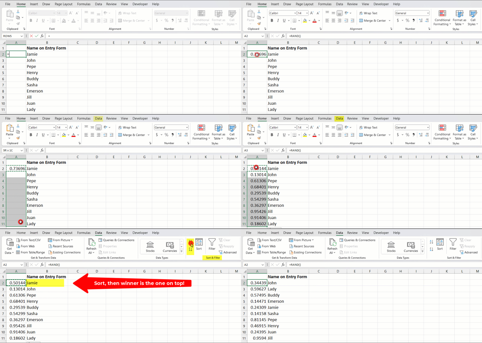
One way to shuffle the order of data in a list is by using a combination of the RAND function and the Sort feature.

With this combination, you can reorder your list by sorting it using the random values generated by the RAND function.

TIP: To select a winner, once you’ve sorted the list by the random values, select the item that is now on top.

To shuffle your list in Excel:

1. Type =RAND() in a cell adjacent to the first item on your list
   1. This will generate a random number between 0 and 1
2. Copy the RAND() function and paste it so that each item on your list has a random value next to it
3. You can now sort the list by the RAND value generated

TIP: To add credibility to the selection process, consider recording a screen capture of the selection using Snagit.

TIP: Because the RAND function is dynamic, once you sort your list, the values will change again. To avoid this, hard-code the results before sorting – copy the random numbers, paste them as values, then sort. This will keep the generated random numbers, but erase the formula.

Create a Formula to Pick an Item from a List

There are different ways that you can combine reference functions to create a formula that will return a random item from a list in Excel.

Using a reference formula eliminates the need to shuffle or reorder your list. All of that will happen automatically as part of the formula calculation.

They all work similarly – by looking through your list and returning an item based on the criteria.

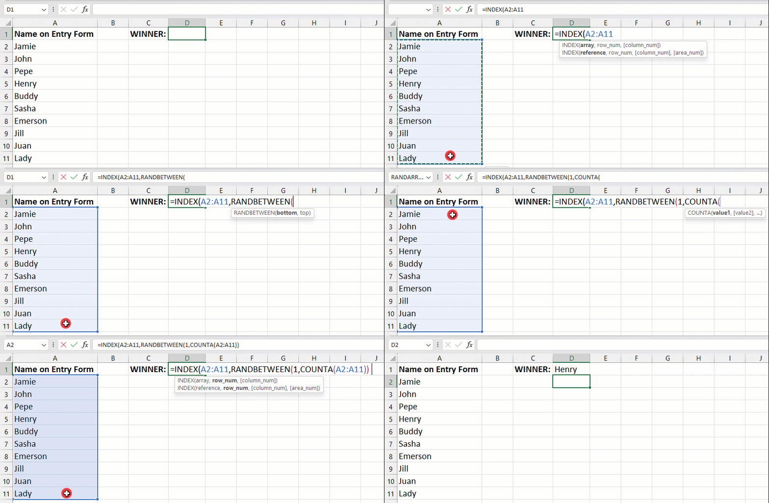
Let’s say we have a list of 10 names from which we need to select one as the winner.

For the example in the gif below, I used the following formula:

=INDEX(List of Names,RANDBETWEEN(1,COUNTA(List of Names)))

TIP: Press F9 on your keyboard to recalculate RANDBETWEEN (and any other dynamic formulas in your workbook) or Shift+F9 to recalculate just the active sheet.

To understand how this formula works it’s easier to examine it starting from its end:

COUNTA

The COUNTA function counts the number of cells that are not empty within a selected area.

For example, if your list contains 10 names, the result of COUNTA would be 10.

TIP: Make sure you do not include the cell with the header/column title in your COUNTA formula!

RANDBETWEEN

RANDBETWEEN generates a random value between the minimum and maximum numbers you set.

By setting the minimum value in the RANDBETWEEN function to 1 and then nesting COUNTA within it, you force RANDBETWEEN to generate a random number between 1 and a maximum of the highest number counted by the COUNTA function.

In this example, because we have 10 names, RANDBETWEEN will select a random number between 1 and 10.

NOTE: Remember that RANDBETWEEN is a dynamic function that refreshes each time a change is made on the sheet; selecting a new winner each time.

INDEX

The INDEX function works by returning whatever is in the cell that is referenced in its criteria.

In this example, we would select the list of names as the data to be searched.

INDEX will then return the name that matches the number generated by the RANDBETWEEN formula.

For example, if the RANDBETWEEN result is 3, then INDEX will return the third name in the list.

Related: What is a Nested Formula in Excel

Other Reference Formulas You Can Use:

As I noted earlier, there are different ways that you can combine functions in Excel to create a formula that will help you select a random item from a list.

In addition to the earlier example, you can try:

• = INDEX(List of Data,RANDBETWEEN(1,ROWS(List of Data)))
• =SORTBY(List of Data,RANDARRAY(ROWS(List of Data)))

Related: How to Use the RANDARRAY Function to Generate Random Data in Excel

And, if your list is numbered (with the numbers being in an adjacent column or row), you can try something like this:

• =VLOOKUP((RANDBETWEEN(1,(MAX select numbered list))),List of Data,2,FALSE)

TIP: If this is something you need to repeat again and again, consider creating a macro for it.

NEXT: Learn how you can customize the sort order of a list in Excel

FYI: This tutorial was created using the desktop version of Excel in Microsoft 365.