UNIQUE Function: Excel’s Unique Values Formula (+ video tutorial)

We may be compensated for your purchase of any of the products featured on this page – it helps us keep the lights on :)

Using the UNIQUE function in Excel is one of the easiest ways to find unique values in your data.

Currently only available to Office 365 users, this function works by returning a list of unique values from your data.

Oh, and you can use it with numbers, letters, and most other characters!

How to Use the UNIQUE Function in Excel

WATCH: How to Use the UNIQUE Function in Exel (Video Tutorial)

When you use the UNIQUE function in Excel, it returns a list of unique values from the data that you’ve selected.

What makes this function so powerful is that it was created in a way to give you options as to *how* you can filter for those unique values – who knew?!

For example, you can set up the UNIQUE function to give you results that:

• List each item in your list once (most common)
• Get unique values whether your data is in columns or rows
• Omit from its results anything that is listed more than once (i.e., returning only items that are not duplicated)

=UNIQUE(array,[by_col],[exactly_once]) – don’t worry if this looks complex, we’ll break this all down below.

Use UNIQUE to Return a List Where Each Item is Listed Once

This is probably the most common way to use Excel’s UNIQUE function.

In this scenario:

• Your items are listed in a column (this means each individual item is in a row in the same column – I know, it seems odd to mention it, but it’s actually really important)
• Some items in your list are repeated
• And you want to generate a list from this where each item is listed only once, even if it’s repeated in the original data

To use the UNIQUE function, you would:

1. Type =UNIQUE(
2. Select the items that you would like to see unique values for (omitting any headers) and
3. Press ENTER

TIP: Make sure to exclude any headers from your UNIQUE function

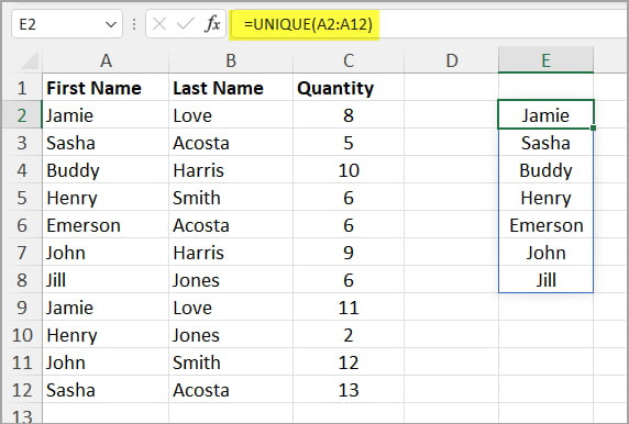
Let’s say you have a list of first names in Column A. The list spans from cells A1 to A12, where A1 is the header.

You would ignore the header and select each of the names to include in your UNIQUE function.

Your formula would look like this: =UNIQUE(A2:A12)

Get a List of Unique Values Whether Your Data is in Columns or Rows

The default for the UNIQUE function is to filter through your data when each list item is in a row (this actually means in a column but in each row of that column).

An example of this would be where a list is in Column A and each item is listed just below it.

This means the items that you would be filtering through are each listed in a separate row (Row 2, Row 3, etc).

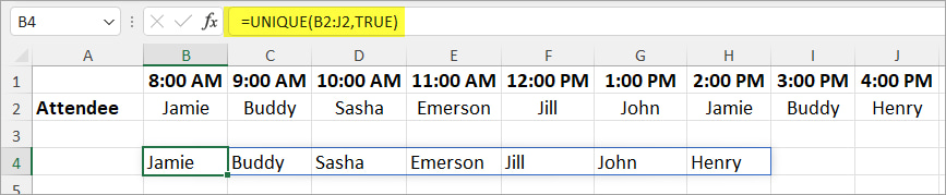
But sometimes, you may need to filter across columns (this means your items are listed across / horizontally but each one is in a different column).

In this case, you would type “TRUE” in the second argument: [by_col]

Your formula would look something like: =UNIQUE(B2:J2,TRUE) or =UNIQUE(B2:J2,TRUE,FALSE)

Use UNIQUE to Get Only Items that Are Not Repeated

You can also use the UNIQUE function to generate a list that omits anything that is listed more than once in your selected data. (i.e., items listed only one time.)

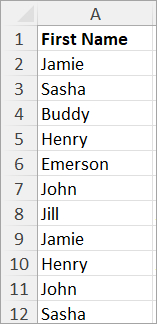
For example, in the list of First Names, only Buddy, Emerson, and Jill appear once. All other items are repeated.

You can use the UNIQUE function in a way that returns only Buddy, Emerson, and Jill.

The option for this can be found in the last argument of the function: “exactly_once”

To do this, in this last argument, you would select (or type) “TRUE.”

To use the UNIQUE function to get items listed only once:

1. Type =UNIQUE(
2. Select your data
3. Skip the second argument, “[by_col],” by inserting 2 commas or selecting FALSE for it (unless you’re filtering across columns, then select TRUE)
4. Select or type TRUE for the third argument “[exactly_once]”

So, for this example, your formula will look like one of two ways:

=UNIQUE(A2:A12,,TRUE) or =UNIQUE(A2:A12,FALSE,TRUE)

If your data is formatted horizontally, your formula might look something like: =UNIQUE(B2:J2,TRUE,TRUE)

Other Cool Ways to Use Excel’s UNIQUE Function

Find Unique Values Across Multiple Columns / Rows

You can use the UNIQUE function to find unique values that span multiple adjacent rows or columns.

For example, say you want to see unique values for first name (Column A) and last name (Column B), not just for the first name.

To do this, you would select both the first name and last name items in your formula.

So your formula might look like: =UNIQUE(A2:B12)

Combine the UNIQUE Function with Other Excel Formulas for More Options

Like other functions in Excel, the UNIQUE function can be combined, or nested, with other functions to generate more custom results.

For example, let’s say that you want to alphabetize the results of your UNIQUE function. You can combine the UNIQUE and SORT functions to do this.

In the example of names that we’ve been using, you would nest the UNIQUE function inside of the SORT function to generate alphabetized results.

Your formula may look like: =SORT(UNIQUE(A2:A12))

---

FYI, this tutorial was created using the desktop version of Excel in Microsoft 365.

---