We may be compensated for your purchase of any of the products featured on this page – it helps us keep the lights on :)
Excel is a powerful tool for working with data, but it’s also loaded with formatting options to help you up the visual appeal of your worksheets. One example is the ability to angle cells – which allows you to rotate the text within cells.
Rotating the text within cells can be particularly useful when you want to fit lengthy labels or elevate the layout of your spreadsheet, for example.
How to Angle Cells in Excel: 2 Easy Ways
Click to Watch: Excel tutorial on how to angle cells in Excel
1. Use the Format Cell Alignment to Angle Cell Contents
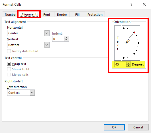
You can angle or rotate the content within cells in your spreadsheet by selecting the cell(s) that you want to rotate the text for, then:
- Right-click and select “Format Cells”
- In the Format Cells window, go to the “Alignment” tab
- In the “Orientation” box, move the guide to the angle you’d like to rotate the text to
You can also type the degree of the rotation in the “Degrees” field box if you know what you’d like it to be.

- Click “OK” to apply the angle formatting
The contents of the cells you selected should now be rotated to the angle that you selected.
2. Rotate Cell Content by Using the Orientation Shortcut in the Ribbon
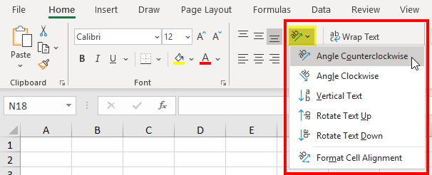
An even easier way to angle cells in Excel can be found in the Home tab, in the Alignment section.

Click on the icon with the diagonal “ab” (this is the Orientation shortcut) and choose one of the preset formats or click on “Format Cell Alignment”, which takes you back to the first option we looked at.

Rotated text can then be formatted with colors, shading, fonts, borders, etc just like other text in your spreadsheet.
NEXT: Learn Ways to Add a Zero Before a Number in Excel (+ video tutorial)

Hello it’s my pleasure to be acquinted with your lessons, pls. I want to learn more about equations in excel sheets
Thank you