How to Make Graph Paper in Excel (+ video tutorial)

We may be compensated for your purchase of any of the products featured on this page – it helps us keep the lights on :)

Is it possible to make graph paper in Excel that you can print? After all, a spreadsheet is just a bunch of grids.

Yet, if you tried to make grid paper in Excel, you probably realized it’s a bit trickier than it seems. That’s because you can’t print only the gridlines:

• You’ll get an error that the sheet is blank.
• You’ll get the same error if you try to add only borders and print.

So, is it even possible to make graph paper using Excel??? YES! And here’s how:

How to Make Printable Graph Paper Using Excel

Watch the Tutorial: How to Make Graph Paper in Excel

1. Set Your Workbook View to Page Layout

First, it’s a good idea to switch your page view to Page Layout. This will make it easier to resize your cells.

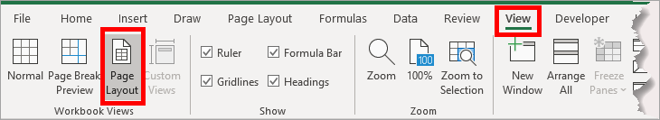
In other page views, Excel cells are measured in points.

You could calculate what the conversion would be from points to inches or centimeters, but, in Page Layout view, you don’t have to worry about that. In this view, you can resize cells using common types of measurements.

2. Insert a Table to Create the Grids for the Graph Paper

Next, select a good portion of the page and insert a Table. The Table will provide the grids for your graph paper.

You can insert a Table either by pressing Ctrl+T on your keyboard or from your Ribbon in the Styles section of your Home tab.

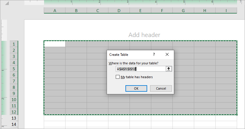
Don’t worry that the Table doesn’t fit to exactly a page right now, you’ll fix this in a moment.

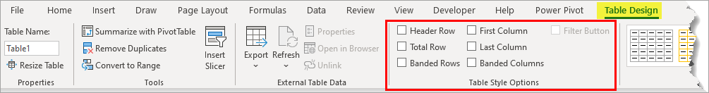
Whenever your cursor is within the Table area, you’ll see a Table Design menu in your Ribbon. In this menu, go to the Table Style Options section and deselect any options that may be checked off.

3. Resize the Cells for the Grid

After you insert the Table, you can resize the cells.

NOTE: If you resize the cells before inserting the Table, they’ll reset after you add the Table, so you’ll want to make sure to do it in this order.

Using Ctrl+A, select all the cells on the sheet (you may need to press Ctrl+A twice).

Then, with all the cells selected, place your cursor along the letter labels of the Columns, right-click and select Column Width to resize the columns.

Enter the measurement you want to use for your grid boxes. In this example, I’m using 0.25”.

TIP: If you’re not in Page Layout view, you will not be able to resize using common measurements (inches or centimeters)

With all the cells still selected, place your cursor along the numerical labels for the Rows, right-click and select Row Height to resize the rows.

TIP: Make sure to set both your Columns and Rows to the same measurement to create perfect squares.

4. Size the Table to Fit the Page

Next, you’ll need to fit the Table to the printable area of the page.

You may, first, need to delete the first row. If you had to deselect Table Headings earlier, you may now have an empty row at the top of your page. Just delete it.

Next, scroll to the end of your Table and, when you see the small triangle at the bottom right corner of the Table, simply drag to the area that you want to cover with the Table.

5. Add Color to Your Gridlines

Your grids may already have color, depending on the Table Style you’re using. But, if not, and you have a color printer and want to add a little color, you can do so from the Table Design menu on the Excel ribbon. Once there, select a colored design with borders around all cells.

Your Excel graph pager sheet is now ready for printing!

---

---